Supplementary data for generation of SAS models

This notebook contains the supplementary data to reproduce the data for JOSS Paper

1. Data Creation

The data for Small Angle Scattering (SAS) was generator using model-generator-sans* library developed by Oak Ridge National Laboratories (ORNL).

*https://www.oclcproxy.ornl.gov/sans-ldrd/model-generator-sans

1.1 Installation:

model-generator-sans was cloned from the repository and was installed using following method:

conda env create -f play_27_env.yml

conda activate playground-27

python setup.py install

1.2 Data Generation

Following four models were selected for our hypothesis evaluation:

• Sphere
• Core-shell-sphere
• Ellipsoid
• Cylinder

For each model, 10000 data files were generated. The example code for data generation is shown below:

• Selection of yaml file to describe the model parameters

  model_file = os.path.join('../', 'tests', 'models', 'sphere.yaml')
  

• Path for Data Generation

  output_dir = os.path.join('../datapath/')
  

• Data Generation

  KNN_gendata.generate(model_file, 10000, output_dir=output_dir)
  

• Importing data from the npy files

  model_name = 'sphere'
  

  with open(os.path.join(output_dir, "%s_par_names.json" % model_name), 'r') as fd:
          par_names = json.load(fd)
  

  q = np.load(os.path.join(output_dir, "%s_q_values.npy" % model_name))
  

  train_data = np.load(os.path.join(output_dir, "%s_data.npy" % model_name))
  

  train_pars = np.load(os.path.join(output_dir, "%s_pars.npy" % model_name))
  

The data and parameters were stored in .csv and .txt files, respectively.

2. Configuration files

YAML configuration files for transformation and machine learning are available in examples folder.

3. Classification using HARDy

The package was uploaded on HYAK HPC Facility at University of Washington. The HPC is equipped with NVIDIA TESLA P100 GPU which was used for training and testing of machine learning models.

from hardy import *

raw_data_path= './data_path/'
tform_config_path= './tform_config.yaml'
classifier_config_path='./classifier_config/'

hardy_main(raw_data_path, tform_config_path, classifier_config_path, batch_size=64, num_test_files_class=750, target_size=(100,100), iterator_mode='arrays',scale=0.2, seed=5,  n_threads=28, classifier='tuner', classes=['ellipsoid', 'sphere', 'core_shell', 'cylinder'], project_name='scat_rgb')

4. Data Analysis

The post-training and testing of data was analyzed using the report-generation module in the hardy. Following script was used to build error-loss and parallel coordinate plots.

from hardy import reporting

Using TensorFlow backend.

loss_accuracy, parallel = reporting.summary_report_plots('../raw_datapath/project_name/')

loss_accuracy.show()

Note: The above image is just an example. The graph generated by HARDy is interactive

parallel.show()

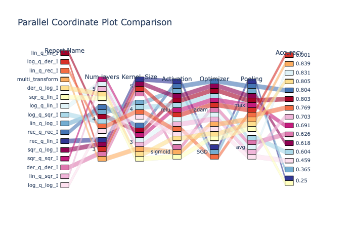
Note: The above image is just an example. The graph generated by HARDy is interactive

5. Validation

The evaluate the effectiveness of machine learning model, the test set files were fitted with most probable classifications using sas-models*.

*https://github.com/SasView/sasmodels

The parameter space used to fit the scattering data for each classification is shown below:

5.1 Sphere

label = "sphere"
pars = dict(scale=1.0, background=0.001,)
kernel = load_model(label)
model = Model(kernel, **pars)

# SET THE FITTING PARAMETERS

model.radius.range(0.0, 3200.0)
model.sld.range(-0.56, 8.00)
model.sld_solvent.range(-0.56, 6.38)
model.radius_pd.range(0.1, 0.11)
experiment = Experiment(data=data, model=model)
problem = FitProblem(experiment)
result = fit(problem, method='dream')
chisq = problem.chisq()

5.2 Core-shell-sphere

label = "core_shell_sphere"
pars = dict(scale=1.0, background=0.001,)
kernel = load_model(label)
model = Model(kernel, **pars)

# SET THE FITTING PARAMETERS

model.radius.range(0.0, 1000.0)
model.thickness.range(0.0, 100.0)
model.sld_core.range(-0.56, 8.00)
model.sld_shell.range(-0.56, 8.00)
model.sld_solvent.range(-0.56, 6.38)
model.radius_pd.range(0.1, 0.11)
experiment = Experiment(data=data, model=model)
problem = FitProblem(experiment)
result = fit(problem, method='dream')

5.3 Cylinder

label = "cylinder"
pars = dict(scale=1.0, background=0.001,)
kernel = load_model(label)
model = Model(kernel, **pars)

# SET THE FITTING PARAMETERS

model.radius.range(0, 1000.0)
model.length.range(0, 1000.0)
model.sld.range(-0.56, 8.00)
model.sld_solvent.range(-0.56, 6.38)
model.radius_pd.range(0, 0.11)
experiment = Experiment(data=data, model=model)
problem = FitProblem(experiment)
result = fit(problem, method='dream')

5.4 Ellipsoid

label = "ellipsoid"
pars = dict(scale=1.0, background=0.001,)
kernel = load_model(label)
model = Model(kernel, **pars)

# SET THE FITTING PARAMETERS

model.radius_polar.range(0.0, 1000.0)
model.radius_equatorial.range(0.0, 1000.0)
model.sld.range(-0.56, 8.00)
model.sld_solvent.range(-0.56, 6.38)
model.radius_polar_pd.range(0, 0.11)
experiment = Experiment(data=data, model=model)
problem = FitProblem(experiment)
result = fit(problem, method='dream')

The source code of automated fitting with csv file creation is available in the examples folder as fit_scattering.py