Feature Mapping
This notebook guides the user through the feature mapping modules we provide in HARDy to evaluate the features through each layers of a trained model
Please note that the feature mapping is only available on MASTER branch due to unavailabiliy of the continous integration tool. In version 1.1, it will be available through conda install
[2]:
import hardy
import os
import matplotlib.pyplot as plt
import numpy as np
Using TensorFlow backend.
Step 1: Importing saved trained model
[3]:
trained_model = hardy.save_load_model('./best_model.h5', load=True)
2021-12-17 11:18:10.735085: I tensorflow/core/platform/cpu_feature_guard.cc:143] Your CPU supports instructions that this TensorFlow binary was not compiled to use: AVX2 FMA
2021-12-17 11:18:10.752896: I tensorflow/compiler/xla/service/service.cc:168] XLA service 0x7fde9f65c800 initialized for platform Host (this does not guarantee that XLA will be used). Devices:
2021-12-17 11:18:10.752911: I tensorflow/compiler/xla/service/service.cc:176]   StreamExecutor device (0): Host, Default Version
Step 2: Extraction of example data set
[4]:
!tar -xzf new_data_set.tar.gz
Step 3: Applying transformation on data set
- Defining the transformation configuration path. For best results, It should be same transformation on which CNN model has been trained
[5]:
transformation_config_path = './scattering_tform_config.yaml'
- Sorting out for
.csvfiles only in the extracted example data set
[6]:
new_data_file_list = [item for item in os.listdir('./new_data_set/') if item.endswith('.csv')]
- Loading the transformation configuration into the notebook
[7]:
tform_command_list, tform_command_dict = hardy.arbitrage.import_tform_config(transformation_config_path)
Successfully Loaded 1 Transforms to Try!
- Defining the parameters required for transformation. The
scaleandtarget_sizeshould be same on which CNN model has been trained
[9]:
run_name = 'log_q_der_I'
new_datapath = './new_data_set/'
classes = ['sphere', 'cylinder', 'core-shell', 'ellipsoid']
project_name = 'feature_maps'
scale = 0.2
target_size = (100, 100)
- Running the transformations
[10]:
hardy.data_wrapper(run_name=run_name, raw_datapath=new_datapath, tform_command_dict=tform_command_dict,
                   classes='d', scale=0.2)
Loaded  44 of 44        Files    at rate of 475 Files per Second
         Success!        About 0.0 Minutes...
Making rgb Images from Data...  Success in 1.64seconds!
That Took 1.8 Sec !
[10]:
0
[11]:
transformed_data = hardy.handling.pickled_data_loader(new_datapath, run_name)
- Selecting one image from the data set
[12]:
image_1 = transformed_data[0][1]
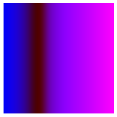
- Plotting the image to see if the RGB transformation has been properly performed
[13]:
plt.imshow(transformed_data[0][1])
plt.axis('off')
[13]:
(-0.5, 99.5, 99.5, -0.5)
- Generating the summary of trained model to verify the outputs or CNN structure
[14]:
trained_model.summary()
Model: "model"
_________________________________________________________________
Layer (type)                 Output Shape              Param #
=================================================================
input_1 (InputLayer)         [(None, 100, 100, 3)]     0
_________________________________________________________________
conv2d (Conv2D)              (None, 100, 100, 18)      504
_________________________________________________________________
conv2d_1 (Conv2D)            (None, 100, 100, 36)      5868
_________________________________________________________________
conv2d_2 (Conv2D)            (None, 100, 100, 54)      17550
_________________________________________________________________
conv2d_3 (Conv2D)            (None, 100, 100, 72)      35064
_________________________________________________________________
global_max_pooling2d (Global (None, 72)                0
_________________________________________________________________
dense (Dense)                (None, 4)                 292
=================================================================
Total params: 59,278
Trainable params: 59,278
Non-trainable params: 0
_________________________________________________________________
Step 4: Generating Feature Maps
The feature_map function requires following parameters: * an image array * trained model * Number of classes on which model is trained * layer num from which you want to see the output * save argument to save the feature maps on disk
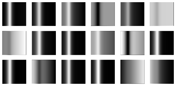
Plotting featuremap for specific layer
[16]:
featuremap = hardy.feature_map(image_1, trained_model, 4, 100, layer_num=1, save=False)
The output is from layer 1, conv2d with shape (None, 100, 100, 18)
Feature prediction from last layer
[17]:
featuremap = hardy.feature_map(image_1, trained_model, 4, 100, layer_num='last', save=False)
The output from final layer is [[3.5393469e-02 6.4015883e-05 6.0268473e-03 9.5851564e-01]]
Please note that the layer_num is changed from integer value to string value of last to get the output from final layer
Plotting feature maps from all Convolutional Layers
[18]:
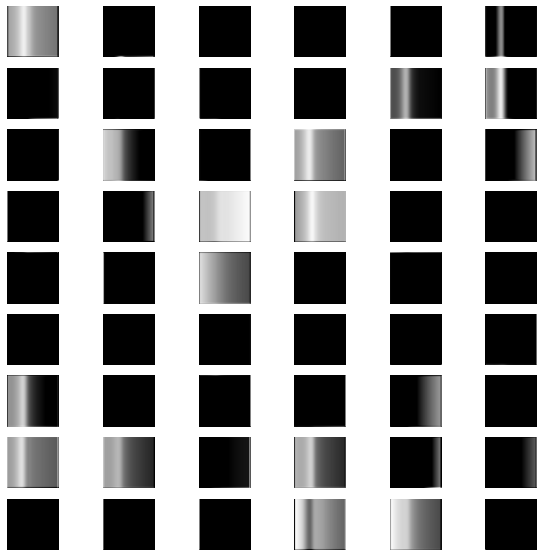
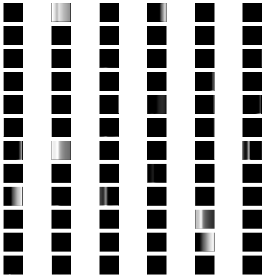
featuremap = hardy.feature_map(image_1, trained_model, 4, 100, save=False)
The output is from layer 0, input_1 with               shape (None, 100, 100, 3)
The output is from layer 1, conv2d with               shape (None, 100, 100, 18)
The output is from layer 2, conv2d_1 with               shape (None, 100, 100, 36)
The output is from layer 3, conv2d_2 with               shape (None, 100, 100, 54)
The output is from layer 4, conv2d_3 with               shape (None, 100, 100, 72)

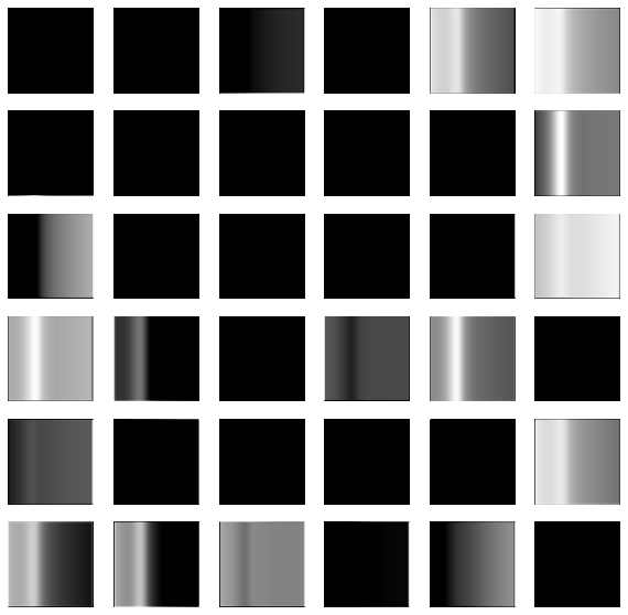
Please note that the layer_num argument hasn’t been used. By default, its value is None